
A blog post covering our recent publication: Christopher W. F. Parsonson, Alexandre Laterre, and Thomas D. Barrett, ‘Reinforcement Learning for Branch-and-Bound Optimisation using Retrospective Trajectories’, AAAI’23: Proceedings of the Thirty-Seventh AAAI Conference on Artificial Intelligence, 2023
Branch-and-bound solvers for combinatorial optimisation
Formally, ‘combinatorial optimisation’ (CO) problems consider the task of assigning integer values to a set of discrete decision variables, subject to a set of constraints, such that some objective is optimised. In practice, this is an important problem class arising in many areas underpinning our everyday lives, from logistics and portfolio optimisation to high performance computing and protein folding.
Whilst many combinatorial problems fall into the NP-hard complexity category (the hardest-to-solve problems in computer science), there are exact solvers available (i.e. those guaranteed to eventually find the optimal solution), with the famous branch-and-bound algorithm standing out as the de facto leading approach.
Proposed in 1960, branch-and-bound is a collection of heuristics which increasingly tightens bounds on the possible values of the decision variables in which an optimal solution can reside until, eventually, only a single (provably optimal) solution is found. It typically uses a search tree, where each node represents a different set of constraints on the variables, along with the corresponding bounds on the objective value. An edge represents ‘partition conditions’ (the added constraints) between nodes. As summarised in Fig. 1, at each step in the algorithm, branch-and-bound performs the following stages: (1) Select a node in the tree. (2) Select (‘branch on’) a variable to tighten the bounds on the sub-problem’s solution space by adding constraints either side of the variable’s current value, generating two child nodes with smaller solution spaces. (3) For each child, solve the dual (integer constraints relaxed) and, where appropriate, the primal (integer constraints applied) problems. (4) Fathom (block off from further exploration) any children which provably cannot contain an integer-feasible solution better than the incumbent. This process is repeated until a provably optimal solution to the original problem is found.

The above heuristics (i.e. the primal, branching, and node selection methods) at each stage jointly determine the performance of branch-and-bound. Among the most important of these to solve efficiency and scalability is branching (which variable to use to partition the focus node’s search space), and was the focus of our work.
Applying machine learning to branch-and-bound solvers
Most state-of-the-art branching algorithms are hand-crafted heuristics which use indicators such as previous branching success and one-step lookaheads to estimate which variable is most promising to branch on in a given state. However, there is no known ‘optimal’ branching policy, and the most performant of these heuristics are too computationally intensive to be used for solving practical problems. Learning high-quality but computationally-fast heuristics with machine learning is therefore an attractive proposition.
To date, the most successful approach to learning-to-branch has been imitation learning with a graph neural network. Concretely, as shown in Fig. 2, the variables and constraints of the focus node (sub-problem) being branched at are represented as a bipartite graph. A graph neural network is then trained to take this encoded bipartite state as input and predict which variable a strong but computationally slow expert branching heuristic would have chosen. The expert imitated is typically strong branching; the best-known algorithm for making the highest quality branching decisions and minimising the final tree size. Imitation learning has been able to get close to the decision quality of this expert. However, the imitation agent avoids the need to explicitly execute computationally expensive operations and instead performs one neural network forward pass to select a branching candidate. Consequently, imitation learning has achieved dramatically faster per-step inference times, reducing the overall branch-and-bound solve time by orders of magnitude relative to the strong branching expert it learned from.

The drawbacks of using imitation learning include needing an expensive data labelling phase, the maximum attainable decision quality being capped by that of the sub-optimal expert being imitated, and the inability to maximise the performance of an expressivity-constrained neural network. Reinforcement learning (RL) can address these shortcomings with the potential to learn novel branching policies from scratch which can exceed the performance of human-designed heuristics. However, prior attempts to apply RL to branching have struggled to cope with the large state-action spaces, partial observability, and long episodes which result in reward sparsity, difficult credit assignment, and high variance returns.
‘Retro branching’: Our method for training state-of-the-art RL branch-and-bound solvers
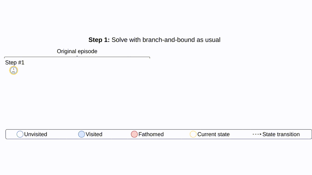
To alleviate the issues of long episodes, large state-action spaces, and partial observability, we propose retro branching (see Fig. 3). During training, we first solve the problem with branch-and-bound as usual but, before storing the episode transitions for the agent to learn from, we retrospectively select each subsequent state transition to construct multiple trajectories from the original episode. Each trajectory consists of sequential nodes within a single sub-tree, allowing the brancher to learn from shorter trajectories with lower return variance and more predictable future states. Whilst the state-action space is still large, the shorter trajectories implicitly define more immediate auxiliary objectives relative to the tree. This reduces the difficulty of exploration since shorter trajectory returns will have a higher probability of being improved upon via stochastic action sampling than when a single long episode is considered. Furthermore, retro branching is compatible with any node selection heuristic, enabling it to be applied to complex combinatorial problems which require sophisticated node selection policies for branch-and-bound to be useful.
We evaluated our approach on four combinatorial tasks (set covering, combinatorial auction, capacitated facility location, and maximum independent set). As shown in Fig. 4, retro branching outperformed the previous state-of-the-art RL branching algorithm, FMSTS, by 3-5x, and came within 20% of the best imitation learning method’s performance.

We believe that this work is an important step towards developing RL agents capable of discovering branching policies which exceed the performance of the best known heuristics today. However, exceeding the performance of imitation agents and the most performant branching heuristics with RL remains an open challenge. Promising areas of further work include combining node and variable selection to reduce partial observability, designing a reward function which accounts for the highly variable influence of branching decisions at different levels in the tree, and going beyond stochastic exploration to increase the likelihood of discovering improved trajectories in large state-action spaces.
All code associated with this project has been open sourced on GitHub.
At InstaDeep, we are committed to continue pushing the boundaries of machine learning research and applications – if you would like to be a part of this journey, check out our opportunities at www.instadeep.com/careers.