Multi-Agent Reinforcement Learning for Resource Balancing in Marine Transportation

With the continuous growth of the global economy and markets, resource imbalance has risen to be one of the central issues in real logistic scenarios. In particular, we focus our study on the marine transportation domain and show how Multi-Agent Reinforcement Learning can be used to learn cooperative policies that limit the severe disparity in supply and demands of empty containers.

Nowadays, marine transportation is crucial for the world’s economy: 80% of the global trade is carried by sea¹. Moreover, most of the world’s marine cargo is transported in containers. In 2004, over 60% of the total amount of goods shipped by sea were containerized, while some routes among economically strong countries are containerized up to 100%². When using such methods to convey goods, problems arise due to the joint combination of the inner nature of container flow with the imbalance of global trade between different regions. For instance, once the freight has been delivered from an exporting country to an importing one, the laden will turn into empty containers that need to be repositioned to satisfy new goods requests in exporting countries.

Empty Container Repositioning (ECR) can be a very costly activity in complex logistic networks and, even if it does not directly generate income, it can account for about 20% of the total costs for shipping companies³.
It is thus clear that building efficient strategies to solve ECR problems is a crucial point for real-world logistic scenarios.

Traditionally, ECR problems were solved with Operation Research (OR) approaches⁴. However, many characteristics of the task at hand make these sorts of approaches unsuitable⁵. More specifically, the following issues arise:

• Uncertainty in the environment. The problem presents different sources of randomness such as the distribution of future orders and the time taken by a given vessel to travel a certain shipping lane. Since OR methods typically generate a plan taking into consideration forecasts on a long period, errors in the estimates of future unknown quantities will accumulate, thus leading the method to sub-optimal behaviors.
• State change of containers. As previously said, while the system is operating, containers will change their state from laden to empty and vice versa. Taking this behavior into account while modeling the problem as a Mixed-Integer Linear Program is complex. Indeed, how this change of state happens in real-world scenarios is completely under the control of business operators whose behaviors are non-linear and black-boxed. For instance, regional policy regulations might introduce delays according to different situations.
• Atomicity of the orders. In real problems, it is reasonable to assume customers’ orders to be atomic. In practice, this means that if a shipping company cannot satisfy an entire customer order, the said custom will probably turn to another shipping company. Modeling such behavior complicates the formulation of the LP problem significantly.

For these reasons, we investigate an alternative approach: Multi-Agent Reinforcement Learning (MARL)⁶. Indeed, by exploiting these Machine Learning tools, we can deal with black box behaviors such as state change of containers and order atomicity while mitigating error propagation due to uncertainty in the environment. Note that in principle, one might adopt approaches based on stochastic programming⁷; however, their computational complexity is far from competitive w.r.t. MARL models.

The rest of the article is structured in the following way. After a short introduction to a tool that we used in our experimentation (i.e., MARO⁸), we dive into the details of Multi-Agent Reinforcement Learning. We propose a novel MARL algorithm that can be used to solve ECR problems and that achieves state-of-the-art performances. Finally, we present and discuss experimental results. We also show a visualization of the learned policy on complex global trade environments.

1. Multi-Agent Resource Optimization Framework

“Multi-Agent Resource Optimization (MARO) platform is an instance of Reinforcement learning as a Service (RaaS) for real-world resource optimization. It can be applied to many important industrial domains, such as container inventory management in logistics, bike repositioning in transportation, virtual machine provisioning in data centers, and asset management in finance. Besides Reinforcement Learning, it also supports other planning/decision mechanisms, such as Operation Research.“

— MARO’s official documentation

The framework, published by Microsoft, contains several appealing features for researchers and companies that want to conduct experiments on a list of problems. Indeed, it provides A) support for distributed training; B) strong visualization tools that can be used to visualize the policy that our agents learn; C) different environments, among which a simulator for marine transportation.

The environment on which our work is focused is Container Inventory Management (CIM). MARO provides the designer with different logistic networks on which you can test your methods. Simple toy domains are available together with global trade scenarios (Figure 1).

The CIM environment is event-driven: when vessels arrive at a given port, the agent retrieves a snapshot of the environment that is used to build its state; then, according to the state, an action will be produced. The action encodes how many empty containers should be discharged (loaded) from (on) the vessel according to the available empty containers at the arrival port and the empty space of the vessel.

A more detailed description of the simulator and the resource flow can be found here.

2. Multi-Agent Reinforcement Learning

Now, let’s see how we can use Multi-Agent Reinforcement Learning and MARO to solve ECR problems.

First, we precisely state the problem setting by defining the entities involved together with a clear goal. Then, it follows a summary of related works that make use of MARL systems to solve ECR problems. Finally, we discuss our approach to the problem, highlighting similarities and differences with state-of-the-art algorithms.

2.1 Problem setting

The ECR problem we are trying to solve can be formalized as a logistic network G = (P, R, V), where P, R, V are the set of ports, routes and vessels respectively. More specifically:

• Each element Pᵢ represent a port. Ports are defined by a location in the network and the number of empty containers in their stocks. Goods demands between two ports in G are generated according to unknown market distributions; supplies, on the other hand, happen when vessels with laden arrive at a given port: the laden will be discharged and those empty containers will turn into empty in the next few days according to black-boxed business logics.
  During each day, a port can satisfy (parts of) the demand using empty containers that are present in its stock on the previous day. If this amount is not enough, container shortages will occur.
• Each route Rₖ is a directed cycle of consecutive ports Pᵢ in the logistic network.
• Each vessel Vⱼ is specified by a duration function that specifies the number of days to traverse a given shipping lane and a container capacity that describes the number of containers that it can transport. Each vessel is also associated with a tuple (Rₖ, Pᵢ), where Rₖ is the route that the vessel is following and Pᵢ is the starting port of the vessel at the beginning of the interaction with the environment.

In ECR problems, the final goal of the agent is to minimize the shortage.

There exists multiple possibilities to cast this problem into a MARL system. For instance, in MARO, each of the different ports corresponds to a different agent. Other works⁵, instead, assume each vessel to be a different agent.
Once this decision is taken, features of the vessels and ports (e.g., vessels’ empty capacity, ports stocks, historical summaries) will serve as a state for the agents. An action (i.e., load/discharge of empty containers) will be taken according to some neural network model whose output is conditioned on the state.

2.2 Related works

The use of MARL systems to solve ECR problems is not new and has been studied and analyzed in different works. Below, we briefly summarize the most relevant to our study.

• Diplomatic Awareness MARL⁵. Here, the authors consider each vessel as an agent with its own independent neural network. Each model is trained with DQN⁸. The state integrates information of current vessel and port with statistical information from neighboring routes. The reward is defined by shortages of the current port together with shortages that occur in neighboring ports.
  This method is not directly supported within MARO since the agent perspective is different (here, each vessel is an agent).
• EncGAT-PreLAC¹⁰. Here, the authors consider each port as an agent; the weights of the network of each agent are shared so to make the overall framework inductive. The model first encodes the features of neighboring entities (port and vessels) using a graph attention mechanism; this encoded state is then used by an Actor-Critic algorithm¹¹. The authors also train the agents in multiple steps. First, agents are pre-trained to maximize their interests. This phase allows the agents to extrapolate and understand the business logic of the problem. Then, a fine-tuning stage takes place: here, a global reward that takes into account shortages of the whole network is adopted.

Other works have also been conducted¹², but they consider a different ECR environment w.r.t. the one that MARO provides.

2.3 Our approach

We built our approach incrementally. In particular, we selected components from relevant methods and introduced new ones based on our intuition on the problem. In the rest of this chapter, we discuss the model we adopted and the optimization scheme that is used to train the agents.

2.3.1 The model
We decided to take a fully observable approach to the MARL system. In particular, the state is composed of relevant features taken from all the ports and vessels belonging to the logistic network. This approach is justified in this sort of problem since it is reasonable to assume that a shipping company, at each time step, has full information on features of its vessels (e.g., empty capacity, speed, expected arrival time, future stops) and ports (e.g., current stock information and historical summaries). In other words, there are negligible communication problems and the state is fully observable.
When adopting this sort of approach, the main concern is scalability. Indeed, as soon as the number of ports and vessels increases, the dimension of the state grows as well. To mitigate this problem, we adopt two small neural networks g(∙ |θₚ) and h(∙| θᵥ) parameterized by θₚ and θᵥ at the bottom of our model. Their goal is to project individual features of each port and vessel into a smaller dimension. Once individual features are encoded, they are concatenated and fed to the head of the network f(∙| θ) together with a local state that collects more specific information on the current port and vessel.
This combination of local and “summarized” global features composes the state of the agent and turned out to yield our best empirical performances.
Please, note that θₚ and θᵥ are trained end to end and are shared among all the ports and vessels.

As in [10], we share weights between agents to make the overall framework inductive. Empirically, we have verified that sharing experience between agents leads to higher performances.
Moreover, we should note that in an event-driven scenario, some agents might appear in very few interactions with the environment: gathering enough information for these agents might require a significantly high amount of trajectories. Therefore, being able to exploit data from other agents turned out to be beneficial also in terms of sample complexity.
Since the model needs to be able to distinguish which agent is taking the action, we augment the state with embeddings of ports, vessels, and routes IDs.

Finally, as in related works¹⁰, the output of our model is a discrete distribution over K possible actions. Action 0 means discharging all empty containers from the vessel, while action K-1 means loading all the possible empty containers given the one stocked at the current port and the empty space of the vessel.
Other actions are evenly distributed with a step of 10%. In all experiments, we set K=21. In this way, we are able to reduce significantly the original discrete action space (from ~50000 to 21, where 50000 is the maximum vessel capacity in the environment).
We should note that being the environment event-driven, it is unnecessary to have K * N actions as output (where N is the number of agents). Indeed, in this case, actions are taken only to respond to events.

2.3.2 Optimization
Taking inspiration from prior works¹⁰, we optimize our agents in a two-stage training process. However, differently from [10], we pre-train the agents to minimize intra-route shortages (i.e., shortages among ports that belong to the same route); this introduces from the beginning trivial levels of cooperation within the network. For instance, if we have a route with 1 exporting port and a few importing ones, the importing agents will learn to load empty containers on the vessels already from the beginning of the training process.
Once this pre-training phase is over, we fine-tune the agents to minimize the global shortage of the network.
We also adopt auxiliary safety inventory rewards that incentivize agents to store additional empty containers in their stocks. This can be beneficial when dealing with noisy environments: if unexpected demand peaks happen, the agents have extra empty containers at their disposal that can be used to satisfy unforeseen demand. While, in principle, these sorts of behaviors should be naturally developed by the agents, we found empirical benefits in including them directly in the reward function. More specifically, strong local minima at the beginning of the training process are avoided.

However, we should note that we are training a shared model in a multi-agent environment: different ports might lead to conflicting gradients, i.e., gradients that point in opposite directions. This might lead to a different form of interference while optimizing the model. To mitigate this issue, we adopt PCGrad¹³, an algorithm that has been originally proposed for Multi-Task Learning¹⁴. Consider the following multi-task example in Figure 2.

As the author reports in the original paper, when we combine conflicting gradients with high curvatures and different gradient magnitudes (i.e., deep valleys, a common property in neural network optimization landscapes), “the resulting multi-task gradient might be dominated by a single task, which comes at the cost of degrading performances in other tasks. Further, due to the high curvature, the improvement in the dominating task might be overestimated, while the degradation in performance of the non-dominating tasks may be underestimated”.
Inspired by their work, we treat each agent as a different task; once gradients have been computed, if a conflicting condition is found we project the gradient of agent i onto the normal vector of agent j’s gradient, and vice versa. This turned out to stabilize performances and avoid local minima when optimizing for global shortages.

The whole architecture is trained using PPO¹⁵ .

3. Experiments

3.1 Environments

We report results on two different global trade scenarios.

• Constant order distribution.
  This is similar to MARO’s “global_trade.22p_l0.0” environment configuration. The main difference is that we increased the noise of the order distributions so that inter-day variations are increased. We also reduced the global amount of demand that is generated each day.
• Sinusoidal order distribution.
  This is similar to MARO’s “global_trade.22p_l0.8” environment configuration. Similar to the previous point, we reduce the global amount of demand that is generated each day. This scenario mimics the seasonality of the global markets.

We should note that default configurations are different from the ones of similar papers. More specifically, the global amount of demand that is generated in each day has been reduced to present a more fair comparison to results that are presented in related works¹⁰ (please, note that original configurations are not publicly available).

Below, plots of the total amount of orders in each for both configurations.

In both cases, the environment is composed of 22 ports, 46 vessels, and 13 routes. We run all baselines and environments on trajectories that are 400 environmental ticks long.

We should also note that, although similar, these environments are numerically different from the one of related works. Unfortunately, even if EncGAT-PreLAC¹⁰ is based on MARO as well, their original environment configurations are not publicly available.

3.2 Baselines

We compare our approach to the following methods:

• Random policy. At each event, a random action is taken.
• No-repositioning policy. No containers are repositioned. In other words, for each event, the action taken is to load (discharge) 0 empty containers on (from) the vessel. By comparing any method with this baseline, we can understand how much an ECR-tailored policy can increase the number of orders that the agent is able to satisfy.
• Import/Export heuristic. This simple baseline first estimates if a port is an importing port or an exporting one. This is done by approximating the ratio of imported and exported goods. If this ratio is greater than 1 (less than 1) the port is an importing (exporting) one and the action distribution will be skewed toward loading (discharging) empty containers on (from) the vessel. A particular case holds if the ratio is close to 1: in this case, the action distribution is skewed toward the non-repositioning policy.
  This simple baseline lets us approximate how much the optimal cooperative behavior of a particular problem is trivial. Indeed, if good performances are found, then, any MARL system should perform at least this good. On the other hand, if this heuristic performs badly while a MARL system outperforms it, this is a good sign that the agents have learned cooperative behaviors that are non-trivial.
• OR approach. The OR baseline we consider is different from the one considered in other works¹⁰. For instance, [10] considers a sliding window forecaster to estimate future and uncertain quantities.
  Instead, we first collect a small number of trajectories with the environment (< 100). These data are used to build estimates of demands and vessels arrivals. We then solve the mathematical formulation using estimates of the mean of the relevant quantities (see appendix A in [5] for details on the formulation).
  We believe it is more appropriate to compare MARL systems with this OR baseline since it makes the comparison fair. Indeed, while training the agent, we sample multiple trajectories from the environment. This lets us extrapolate information about the distributions that are governing the underlying phenomenon. To this end, we apply the same reasoning to the OR method and we let it collect information so that it can build more accurate estimates to be used while computing the plan.
• EncGAT-PreLAC¹⁰. Note that we do not directly run their code since it is not publicly available. Given our understanding of the paper, we implemented our own version of the algorithm as well as we could.

3.3 Results summary

The following table summarizes the results of all baselines on both environments. Results are reported in terms of the percentage of satisfied order demands.

Let’s start analyzing the table by comparing simple methods with MARL approaches. As we can see, the non-repositioning policy outperforms the random one, and its performance is significantly better in terms of satisfied demand. This poses a strong local minima that makes the optimization of MARL systems harder. We also note that the Import/Export heuristic reaches performances that are comparable with the non-repositioning one. Therefore, in these environments, simple hand-designed behaviors won’t help in minimizing the shortage significantly. On the other, both our approach and EncGAT-PreLAC are able to find more complex cooperative schemes that lead to better performances.

The final metrics that EncGAT-PreLAC is able to achieve are way lower w.r.t. the ones reported in the original paper¹⁰. The causes of this failure can be many, including and not limited to different environment configurations and bugs in the MARO framework. Indeed, until a few weeks ago there was no noise in the environment: every trajectory was containing exactly the same order amount in each day and vessels’ arrivals at different ports were fixed. This might have led the method to overfitting issues. On the other, we apply noise both to order distribution and vessels’ speed. We also point out that many reproducibility details are missing and the code is not publicly available; therefore, the problem might also be our fault.

Finally, as we can see, the new OR implementation leads to significantly low shortages, in particular in the constant order distribution environment. In this case, indeed, it is clear that the effect of cumulative noise is negligible since each port in the network will always require the same amount of empty containers. When the shape of the order distribution is more complex (i.e., sinusoidal order distribution), noise while planning will take more severe effects. In such situations, our MARL system approach leads to the best results.

3.4 Policy visualization

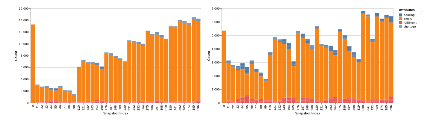
So, what our agents have learned during the training process? Below, we compare relevant port attributes at the beginning (left) and end (right) of the learning process. The scenario that we considered is the sinusoidal one.
The attributes we report per day are:

• Booking: demand.
• Empty: number of empty containers being stocked in each port.
• Fulfilment: number of orders fulfilled.
• Shortage: unsatisfied demand on a given day.

First of all, as one might expect at the beginning of the learning process, random actions are taken. Consider the following picture about the behavior in Singapore (Figure 5). Singapore is a port that imports and exports approximately the same amount of goods.

As we can see, in the beginning, empty stocks are soon loaded onto a vessel: this leads to incur in shortages during the next period. Once the training process is over, instead, the agent has learned to keep empty containers to satisfy future demand.

Ports such as New York (Figure 6), instead, are importing ports that will experience a significant increase of empty containers over time. In this case, it is important to learn cooperative behaviors that distribute these excessive stocks in other ports. This is, indeed, what happens at the end of the training process. You might notice that the scale between the two pictures is different.

Now, what happens to exporting ports? Consider the situation in Bremerhaven (Figure 7). Here, while learning, port stocks are enough to satisfy the demands in the initial period, but, as soon as time passes, the agent has not the ability to properly maintaining stocks during the entire horizon.
Once a cooperative behavior is learned, the agent will discharge empty containers from other vessels to satisfy future demands.

To conclude, we present visualizations (Video 1 and Video 2) of the behavior of the agents in both environments at the beginning and at the end of the learning process. Videos have been generated using the geo-visualization tool provided in MARO.

In each video, we present a slice of an entire trajectory to illustrate the qualitative behaviors of the agents. A small box on the right shows the quantity of fulfilled orders and shortages each day.
On the global map, instead, we can see vessels (white elements) traversing shipping lines to reach their destination port. During each day, a port can assume different colors depending on its status (Figure 8).

References

1. UNCTAD. 2017. Review of maritime transport 2017. OCLC: 1022725798
2. Steenken, Dirk, Stefan Voß, and Robert Stahlbock. “Container terminal operation and operations research-a classification and literature review.” OR spectrum 26.1 (2004): 3–49.
3. Song, Dong-Ping, and Jing-Xin Dong. “Empty container repositioning.” Handbook of ocean container transport logistics (2015): 163–208.
4. Long, Yin, Loo Hay Lee, and Ek Peng Chew. “The sample average approximation method for empty container repositioning with uncertainties.” European Journal of Operational Research 222.1 (2012): 65–75.
5. Li, Xihan, et al. “A cooperative multi-agent reinforcement learning framework for resource balancing in complex logistics network.” arXiv preprint arXiv:1903.00714 (2019).
6. Busoniu, Lucian, Robert Babuska, and Bart De Schutter. “A comprehensive survey of multiagent reinforcement learning.” IEEE Transactions on Systems, Man, and Cybernetics, Part C (Applications and Reviews) 38.2 (2008): 156–172.
7. Long, Yin, Loo Hay Lee, and Ek Peng Chew. “The sample average approximation method for empty container repositioning with uncertainties.” European Journal of Operational Research 222.1 (2012): 65–75.
8. Arthur Jiang et al., “MARO: A Multi-Agent Resource Optimization Platform”(2020) | Github page
9. Mnih, Volodymyr, et al. “Playing atari with deep reinforcement learning.” arXiv preprint arXiv:1312.5602 (2013).
10. Shi, Wenlei, et al. “Cooperative Policy Learning with Pre-trained Heterogeneous Observation Representations.” arXiv preprint arXiv:2012.13099 (2020).
11. Konda, Vijay R., and John N. Tsitsiklis. “Actor-critic algorithms.” Advances in neural information processing systems. 2000.
12. Luo, Qiang, and Xiaojun Huang. “Multi-Agent Reinforcement Learning for Empty Container Repositioning.” 2018 IEEE 9th International Conference on Software Engineering and Service Science (ICSESS). IEEE, 2018.
13. Yu, Tianhe, et al. “Gradient surgery for multi-task learning.” arXiv preprint arXiv:2001.06782 (2020).
14. Zhang, Yu, and Qiang Yang. “A survey on multi-task learning.” arXiv preprint arXiv:1707.08114 (2017).
15. Schulman, John, et al. “Proximal policy optimization algorithms.” arXiv preprint arXiv:1707.06347 (2017).

Thanks to Riccardo Poiani, Alex Laterre and Ciprian Stirbu.